In this post, let us review
As I have discussed in another blogpost, while performing cross-validation in time series, test set should follow the training set because of inherent ordering of observations which is unique to time series data.
We can use TimeSeriesSplit option under sklearn for splitting time series data. For demonstration purpose, I have divided the air passengers dataset into three folds: three training and three testing data sets. The data looks like this:

The total number of observations in the data is 144. Let us now perform the three fold cross-validation by splitting the data using TimeSeriesSplit. Then find out how many values are there in each fold. The number of observations in test set will be generally the same (36 in this case as shown in the below results), while the number of observations in training sets will differ (36, 72 and 108).
In this post, we have seen how to perform cross-validation in time series analysis and what are the forecast accuracy measures. If you have any suggestions or questions, feel free to share.
- Standard statistical measures of forecasting accuracy
- Cross-validation in time series
- How to plot forecasts and,
- How to calculate forecasting accuracy in Python
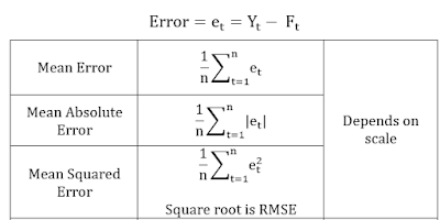
I. Standard statistical measures of forecasting accuracy


Root Mean Square Error (RMSE) and Mean Absolute Percentile Error (MAPE) are the popular measures.
RMSE is scale dependent, that means comparing the RMS errors of two different series measured on different units is not meaningful.
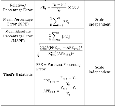
While MAPE is scale independent, however the loss function is asymmetric. What is assymetric loss function? Lets us understand it with an example. Suppose an actual value is 100 while the forecast is 80, MAPE will be (20/100*100) = 20%. However if the forecast is 100 and the actual value is 80 (again the deviation from the actual value is same, 20), then MAPE will be (20/ 80*100) 25%.
One more problem with percentage based measures is that whenever the original values are closer to 0, or 0, accuracy results may be misleading.
II. Cross-validation in time series
As I have discussed in another blogpost, while performing cross-validation in time series, test set should follow the training set because of inherent ordering of observations which is unique to time series data.
a) How to split time series data into tran and test sets?
We can use TimeSeriesSplit option under sklearn for splitting time series data. For demonstration purpose, I have divided the air passengers dataset into three folds: three training and three testing data sets. The data looks like this:

The total number of observations in the data is 144. Let us now perform the three fold cross-validation by splitting the data using TimeSeriesSplit. Then find out how many values are there in each fold. The number of observations in test set will be generally the same (36 in this case as shown in the below results), while the number of observations in training sets will differ (36, 72 and 108).
from sklearn.model_selection import TimeSeriesSplit
#Specify fold and perform splitting
tscv = TimeSeriesSplit(n_splits=3)
tscv.split(data)
#Find out no of observations in train and test sets
i=0
for train, test in tscv.split(data):
    i=i+1
    print ("No of observations under train%s=%s" % (i, len(train)))
    print ("No of observations under test%s=%s" % (i, len(test)))
 |
| Output |
Accordingly split the data into three training (train1, train2 and train3) and test sets (test1, test2 and test3) each using iloc function.
#Splitting according to the above description
train1, test1 = data.iloc[:36, 0], data.iloc[36:72, 0]
train2, test2 = data.iloc[:72, 0], data.iloc[72:108, 0]
train3, test3 = data.iloc[:108, 0], data.iloc[108:144, 0]
#Fit a model
from statsmodels.tsa.holtwinters import ExponentialSmoothing
from sklearn.metrics import mean_squared_error
from math import sqrt

#First fold RMSE
model1 = ExponentialSmoothing(train1, seasonal='mul', seasonal_periods=12).fit()
pred1 = model1.predict(start=test1.index[0], end=test1.index[-1])
RMSE1=round(sqrt(mean_squared_error(test1, pred1)),2)

#Second fold RMSE
model2 = ExponentialSmoothing(train2, seasonal='mul', seasonal_periods=12).fit()
pred2 = model2.predict(start=test2.index[0], end=test2.index[-1])
RMSE2=round(sqrt(mean_squared_error(test2, pred2)),2)

#Third fold RMSE
model3 = ExponentialSmoothing(train3, seasonal='mul', seasonal_periods=12).fit()
pred3 = model3.predict(start=test3.index[0], end=test3.index[-1])
RMSE3=round(sqrt(mean_squared_error(test3, pred3)),2)

print ("RMSE1:", RMSE1)
print ("RMSE2:", RMSE2)
print ("RMSE3:", RMSE3)

Overall_RMSE=round((RMSE1+RMSE2+RMSE3)/3,2)
print ("Overall RMSE:", Overall_RMSE)
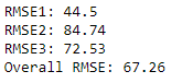 |
| Output: RMSE across different folds and overall RMSE |
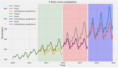
b) Plotting
Let us plot the training, test and forecast values from these three folds.
#Import libraries

import pandas as pd
import numpy as np
import matplotlib.pyplot as plt
from statsmodels.tsa.holtwinters import ExponentialSmoothing
%matplotlib inline
plt.style.use('fivethirtyeight')
from pylab import rcParams
rcParams['figure.figsize'] = 14,8

#Labels and titles
plt.xlabel("Time")
plt.ylabel("Passengers")
plt.title("3 fold cross-validation")

#First fold- CV
plt.plot(train1.index, train1, label='Train1')
plt.plot(test1.index, test1, label='Test1')
plt.plot(pred1.index, pred1, label='Holt-Winters prediction1')
plt.legend(loc='best')
#Highlighting the region
plt.axvspan(test1.index[0], test1.index[-1],  facecolor='g', alpha=0.1)

#Second fold
plt.plot(train2.index, train2, label='Train2')
plt.plot(test2.index, test2, label='Test2')
plt.plot(pred2.index, pred2, label='Holt-Winters prediction2')
plt.legend(loc='best')
#Highlighting the region
plt.axvspan(test2.index[0], test2.index[-1],  facecolor='r', alpha=0.2)

#Third fold
plt.plot(test3.index, test3, label='Test3')
plt.plot(pred3.index, pred3, label='Holt-Winters prediction3')
plt.legend(loc='best')
#Highlighting the region
plt.axvspan(test3.index[0], test3.index[-1],  facecolor='b', alpha=0.3)

I have used the base code from this answer to plot the time series forecasts and modified it to depict the three fold cross validation.
III. Summary
In this post, we have seen how to perform cross-validation in time series analysis and what are the forecast accuracy measures. If you have any suggestions or questions, feel free to share.